How to analytically calculate the system response matrix#
Jiahao Bao, Fang Han
Sept 19, 2024
30 min ~ 1 hour
Here is how to start your jouney in SPEBT project. I’ll offer you a step by step instruction on how to understand and use our python codes. SPEBT is our github website, and spbet.github.io is our project website.
Outline#
Our project, in the code part, aims to develop basic tools for future device development. This involves basically 2 parts:
python mathematical caculation (in the pymatcal module)
python reconstruction (in the pyrecon module)
With these two complete modules, we can quickly design the system matrix and verify its reconstruction performance.
Here are steps before get down on coding.
Read the
.ymlfiles in/spebt/pymatcal/examplesand figure out how we config our virtual system.detector geometry defines a series of boxes by giving the coordinates of two diagnol. It is like: \([x_0,x_1,y_0,y_1,z_0,z_1,n_{detector},\mu_{attenuation}]\). For your mechanical collimator, \(n_{detector}=0,\mu_{attenuation}=10.0\) or other large numbers; for your detector unit \(n_ {detector}=\) your detector number,\(\mu_ {attenuation}=0.48\) for the scintillator material we want to use.
N-subdivision xyz in detector and FOV part defines how fine the voxel or detector unit will be divided for calculation. The finer, the more accurate the result should be, while calculation it self will be slower.
active geometry indices gives the detectors that will be calculated. Remember to change it if you’d like to add more detectors
N-voxels xyz & mm-per-voxel xyz gives the size of FOV.
radial shift means the detector front edge to FOV center distance in radial direction. It is in a list form, so you can do radial shift in one calculation by giving multiple values here.
tangential shift means detector center to FOV center distance in tangential direction. Also, it can be a list.
rotation is a range, basiclly from 0 to 360. Usually you will have to give enough steps to achieve sampling completeness in a system matrix.
Understand the theory of imaging.
The assumption is that \(g=Hf\), where \(H\) is system matrix in 2-D form, \(f\) is the image you want reconstruct. It is flatten into a 1-D vector. \(g\) is the
projection, the signal detected by our detectors. It can be reshaped into asinogramwith one dimension as rotation degrees and the other as ID or relative position of detectors.We want to know \(f\) based on \(g\) and \(H\). \(g\) is got naturally. To get \(H\), we use
First-principles CalculationsorMento Carlo Simulation. The former one is to useray tracing algorithmto caculate the probability of certain pixel emitting \(\gamma\) photon to certain detector in certain position.Since H is not always inversable. We use
MLEM algorithmfor reconstruction. Refer to SPEBT Group Folder. Inrefsyou can view the book chapter Iterative Image Reconstruction.Recognizing we must use MPI(Message Passing Interface) to do parallel caculation.
The reason behind is that just in our code test, we use about 100x100 phantom and 1~5 detectors, rotating 360 degrees, and sample for every 10 degrees. That is 1080000 system matrix elements and 1080000 ray tracing algorithom caculation. So we have to use mpi on a cluster to speed up caculation.
Procedures to use codes#
Before you get your cluster access, you can run the loop version on your own computer.
If you are in the environment of cluster, see spebt.github.io for help.
It is worthy of noting that you can use sbatch to submit muiltiple jobs onto cluster, which will be of good use. See onubccr for detailed instruction.Prepare the environment you need.
Install the modules:
numpy == 1.24.6
pyyaml == 6.0.1
jsonchema == 4.19.2
h5py == 3.11.0
mpi4py == 3.1.6
You can run pip install -r requirements.txt, but when you install h5py and mpi4py, it sometimes goes wrong. Then you trypip install --no-binary=h5py h5py and then reinstall mpi4py. If you still cannot load them, contact your advisor. Of course, you will need other modules, but you should not have problems with that.
If you are to use sbatch to run pymatcal module, try this:
#  On CCR comand line, try
ml intel gcccore/11.2.0 python/3.9.6-bare hdf5/1.14.1
pip install --user mpi4py
# Then the following code (in one line)
CC=mpicc HDF5_MPI="ON" HDF5_DIR="/cvmfs/soft.ccr.buffalo.edu/versions/2023.01/easybuild/software/avx512/MPI/intel/2022.0.1/impi/2021.5.0/hdf5/1.14.1" pip install --user --no-binary=h5py h5py
Try to run the
get_all_ppdfsfiles, either mpi or nonmpi
It uses ray tracing algorithm to caculate our system matrix. See get_all_ppdfs_mpi.py.
You give a configuration to get_all_ppdfs_mpi.py, like test_small.yml, to the programme. The command is like:
mpiexec -n 4 python3 get_all_ppdfs_mpi.py test_small.yml
which means you request 4 nodes to run the programme with the configuration test_small.yml
The output of the python file is a system matrix file in .hdf5 form. .hdf5 is a kind of file supported by h5py module and is used to restore large numpy array or we say, tensor. In fact all our data is restored that way. To use the data in an hdf5 file as a numpy array:
import h5py

with h5py.File('your_file_name.hdf5','r') as f:
   data = f['data_keyname'][...]
And to store your numpy array data in an hdf5 file:
import h5py

with h5py.File(outFname, "w", driver="mpio", comm=MPI.COMM_WORLD) as f:
   #diver and comm are optional, the example here is for MPI
   dset = f.create_dataset("data_keyname", (size_of_dimension0,size_of_dimension1,size_of_dimension2), dtype = np.float64)
If you do not use the with structure, remember to f.close() after f = h5py.File('your_file_name.hdf5','w'), otherwise system will throw an error.
Pay special attention to the definition of your system matrix! One kind of definition is (tangential_shift, radial_shift, rotation_angles, detectors, FOV). For exammple, H[3,50,30,2,8832] is the possibility of the\(\gamma\) photon emitted by the 8832th voxel of FOV being detected by 2nd detctor unit, which has been rotated 30 degrees shifted +50mm radially outward and 3mm tangentially C.C.W. Here tangential_shift, radial_shift and rotation_angles correspond to those in configuration file. The reason for such things is enhanced sampling. In the get_config.py, they are read as lists, so each number in such dimensions refers to a certain postion of your panel.
After that, you can choose to visualize your system matrix
You might use plot_ppdf_hdf5.py, but it is not designed for a seris of rotation angles. A better option is to use jupyter notebook and run read_sysmat_hdf5.ipynb.
You should be able to see weather the sysmatrix is right or wrong by looking at the pictures. The first figure without rotation tells about how much multiplexing we have. The second one shows if your detector covers all the field of view (FOV). Here is an example, which is actuvally not good enough: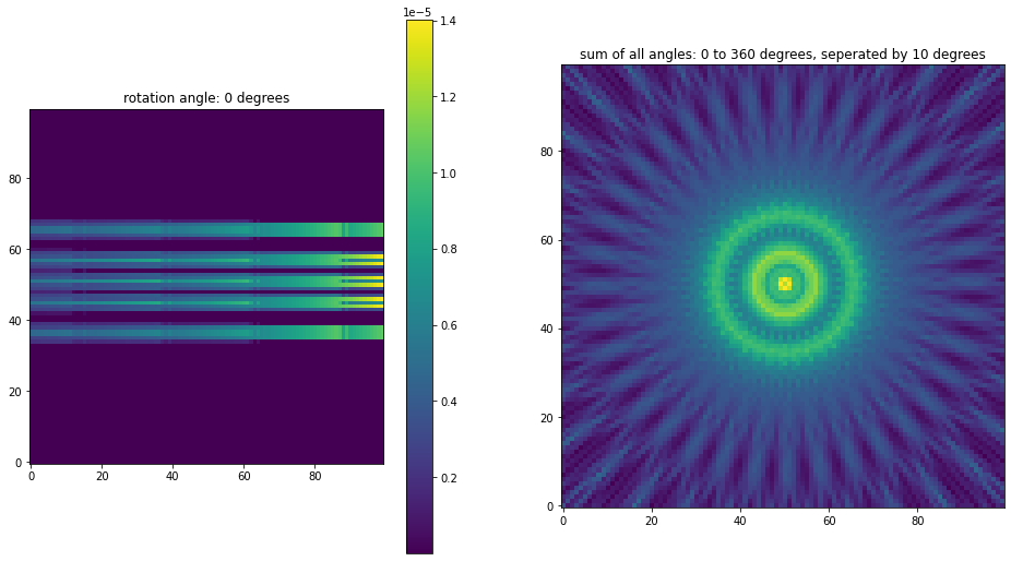
Next you can move to reconstrcution.
Basically, you use the tools in MLEM module: get_forward_projection,get_backward_projection amd reconstruction. The Idea of Maximized Likelihood Expectation Maximization(MLEM) is that the reconstructed image is continuously adjusted with forward-to-backward projection to get the result in an iterative fashion.
In our tests, we use phantom to generate projection. And we compare reconstructed image with phantom to see the quality of reconstruction. Two kinds of phantoms are often used: point source phantom and hot rod pahntom. We have the .npz files in our folder. Reshape them into 1-D vector before reconstruction.
Pay special attention to the dimensions of your system matrix! You need to reshape system matrix into 2-D. The 4 dimensions of tangential_shift, radial_shift, rotation_angles and detectors should be added together using sysmat=numpy.sum(data,axis=(0,1,2)).
We use log-likelihood to determine weather iteration is sufficient. The formula is:
A good way for going on reconstruction is also to use jupyter notebook. We have .ipynb files just for reconstruction in our group project folder.